Supervised Learning with Scikit Learn
Machine Learning is the art of giving computers the ability to learn from data and make decisions on their own without explicitly programmed for example
- The determination of benign and malign according to the tumor size
- Google News Selecting similar news and making a cluster of news which are related
- Classifying emails in the spam or not a spam
- Prediction of house pricing according to the number of rooms, furnishing, age, etc.
- Detection of where a bank transaction is fraud or not
There are many more examples of machine learning, here we are going to discuss Supervised Machine Learning, There are two parts of data features and labels, features are the input for the model just like the size of tumors is if we put the size of tumors the model will tell us whether it is malign or benign, the prediction here whether malign or benign are the labels, there some types of data which does not contain labels such as a grouping of news which are related does not require any labels, but here in supervised learning, we are concerned with data labels, so loosely we can say the Machine Learning modeling with labels are known as supervised learning.
For further understanding, we are going to use iris datasets, which have 4 features Sepal.Length, Sepal.Width, Petal.Length and Petal.Width and one target variable Species
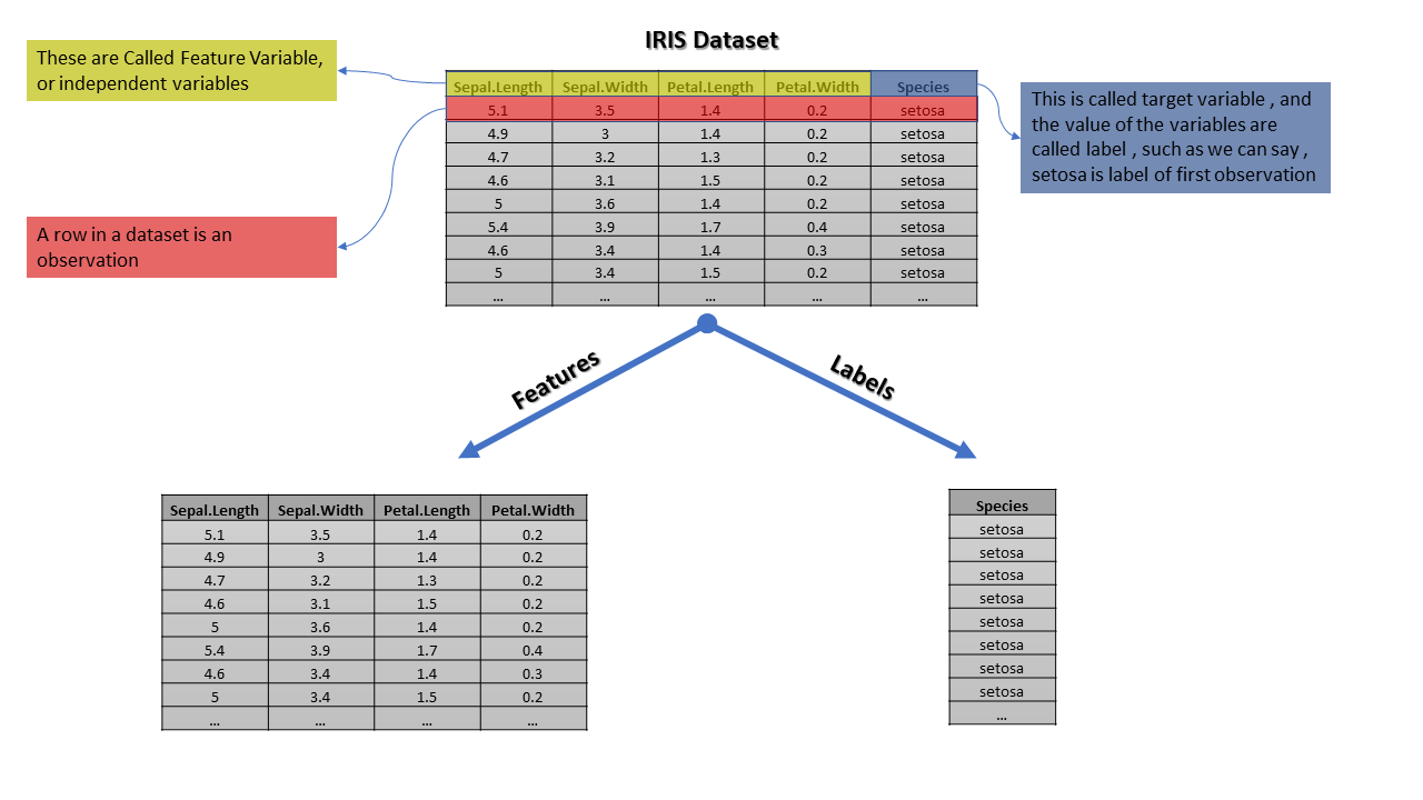
This is a long dataset with labels virginica, setosa and Versicolor however we are representing only part of data so we can see in the target column we have the only setosa
The realization of the target variable is known as labels however most of the data scientists use them interchangeably. The predictor variable and feature are the same thing and also known as the independent variable, while the target variable is known as the dependent variable
Classification
Classification is a machine learning models which classify things , such as classifying mail is spam or not , or in the iris data classifying where the plant is virginica , setosa or versicolor is the classification.
First of all we gonna load our dataset using the following codes, which also imports pandas and numpy under their usual aliases.
from sklearn import datasets
import pandas as pd
import numpy as np
iris = datasets.load_iris()
type(iris)
sklearn.utils.Bunch
We can see that iris dataset is a bunch, bunch is a datatypes which have a key value pairs, we can look at the pairs using following code
print(iris.keys())
dict_keys(['data', 'target', 'target_names', 'DESCR', 'feature_names', 'filename'])
type(iris.data),type(iris.target),type(iris.target_names),type(iris.DESCR),type(iris.feature_names)
(numpy.ndarray, numpy.ndarray, numpy.ndarray, str, list)
We can see that iris.data and iris.target is numpy array , also target names is also an array , DESCR is string and features names is string, if we iris.data.shape and iris.target.shape we can see data has shape 150 rows and 4 columns and this is our features,we can take a look at our data by the command print(iris.data) , similarly the shape of target variable have 150 rows and 1 columns as we expected and we can look at it using print(iris.target) However our target variable is encoded where
- 0 represent setosa
- 1 represent versicolor
- 2 represent virginica
It can be seen using iris.targets and it is also described in iris.descr, let us store iris.data in variable X and iris.target in y
X = iris.data
y = iris.target
Let us construct a dataframe from the X which have header as iris.feature_names and show how our dataframe actuaaly looks like using head() method
df = pd.DataFrame(X , columns = iris.feature_names)
df.head()
| sepal length (cm) | sepal width (cm) | petal length (cm) | petal width (cm) | |
|---|---|---|---|---|
| 0 | 5.1 | 3.5 | 1.4 | 0.2 |
| 1 | 4.9 | 3.0 | 1.4 | 0.2 |
| 2 | 4.7 | 3.2 | 1.3 | 0.2 |
| 3 | 4.6 | 3.1 | 1.5 | 0.2 |
| 4 | 5.0 | 3.6 | 1.4 | 0.2 |
k-Nearest Neighbours
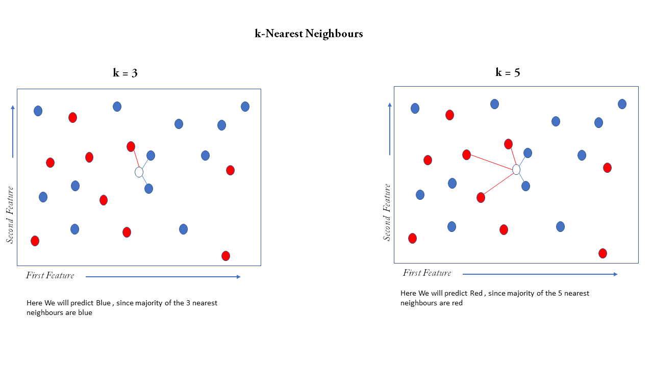
Now let us train our first model using the k-Nearest Neighbors (or kNN), it is quite simple, first suppose there are only two features in our dataset then we can plot each observation (that is a single row in a dataset ) simply on the 2D plane as a point where the first feature is on the x-axis and second feature on the y-axis, and suppose the color of the point is a label that can be red or blue, suppose we get a feature with know label on it only with two features now we can plot that point on the same 2D plane but we cannot determine the color of the point since it is not labeled, now we have to predict label suppose we take 3 nearest observation on the plane then it is kNN with k=3 now we have to take the majority vote of 3 nearest neighbors, 2 of them is blue so our prediction is blue, our prediction may change with change in k, suppose k=5 now out of the 5 nearest neighbors 3 are red and 2 are blue then we predict red
This algorithm can be extended to n features where n number of features is greater than 2, by plotting the points in an n-dimensional euclidean plane and then computing the nearest neighbors
Training and Prediction
In Scikit Learn there are two important methods .fit that will be useful for training the model and .predict to predict the label using a trained model, now to use kNN we have to import sklearn.neighbors from sklearn library using from import KNeighborsClassifier and then we have to initialize it and set the value for k let set it to 5 using KNeighborsClassifier(n_neighbors=5) then we will fit the data using .fit method
from sklearn.neighbors import KNeighborsClassifier
knn_model = KNeighborsClassifier(n_neighbors=5)  #Storing the model in varible knn_model
knn_model.fit(X,y)                               #Fitting ot training the model
KNeighborsClassifier(algorithm='auto', leaf_size=30, metric='minkowski',
                     metric_params=None, n_jobs=None, n_neighbors=5, p=2,
                     weights='uniform')
Now we have trained our model and stored it into the variable knn_model , Now if we have given the sepal length, width, and petal length, we can predict the species let us predict for 4.6,3.8,3.7,0.9 as sepal length, sepal width, petal length and petal width using .predict method
knn_model.predict([[4.4,3.8,3.7,0.9]])
array([1])
Hence we can see we have predicted 1 which represents Versicolor similarly we can do a lot of prediction at once by creating a NumPy array and then passing it as an argument to the knn_model.predict(), we must take care that the number of columns is equal to the number of features that we have used to train the model, now let us see an example
array = np.array([[4.4,3.8,3.7,0.9],
                  [3.2,5.7,2.0,1.3],
                  [5.5,1.9,2.8,4.7],
                  [3.2,9.7,6.2,1.0]])

prediction=knn_model.predict(array)
print(prediction)
[1 0 2 2]
iris.target_names[prediction]
Now we can get decoded species name by passing the prediction to iris.target as an index
array(['versicolor', 'setosa', 'virginica', 'virginica'], dtype='<U10')
Measuring the performance
Now we have trained or model , now we must measure the performance of our model to get the idea of how good or how bad is our model,there are various metric to measure the performance such as Accuracy , Precision , F-Measure etc. but one of the question we have is to which data to use for calculating performance since the data used for training will give too optimistic metric , and may be good only for the data that we have used for training however our main target in machine learning models to train the data such that is predicts the labels for new data, so we need to calculatr our metric on the new data but that is not possible since new data will not be labeled , so a typical operating procedure for a datascientists to split the data into train and test sets where train set will be used for training and the test set will be used for testing and so on calulating the metric such as Accuracy and all we are going to use accuracy here that is equal to the total true prediction divided by toal number of prediction , suppose we 100 observation in test sets and out of them our model predicte 75 of them true , that means there are 75 prediction ehic are right and 25 are wrong so at las t we can say accuracy
Splitting the dataset into Train and Test sets
To split the dataset, first of all, we will import train_test_split from sklearn.model_selection, now the method train_test_split() will take some arguments, the first argument will be feature data and the second will be labels and that will be train_test_split(X,y) however this method will work fine, but to increase the usability of method it can take more arguments such as
- test_size which is a proportion of the test set, default is set to 0.25, which means it will split 25% of the data as a test set and 75% train set however if someone wants test set to be 20% and train set 80% they can use
test_size = 0.2 - random_state it is the seed for the generation of random numbers, look the train_test_split method split the dataset randomly, it does not just take 25% data from the data for the test set, it randomly selects data for test sets, suppose we want in future to generate same train and test set in future for our datasets we can generate same test and train dataset using the same random_state
- stratify argument is “y” if we want our test set to have the same proportion of labels as our dataset, this argument stratify dataset according to the labels, suppose in our iris dataset there are three labels setosa, Versicolor and Virginica Now in this case our dataset will be split into three datasets first containing only those observation whose label is setosa, second with Versicolor and the third with virginica, then it will take 25% of them, randomly from all of them and merge them to create test set, in this way we know the proportion of setosa, Versicolor and viginica is same in the test set and iris dataset
Let us talk about the output of the train_test_split method it will give four arrays, the feature of the train set, the feature of the test set, labels of the train set and labels of the test sets, lets split our dataset, and train our model on the training set
from sklearn.model_selection import train_test_split
X_train , X_test , y_train , y_test = train_test_split(X,y,test_size = 0.25 , stratify=y)
knn_model.fit(X_train,y_train)
KNeighborsClassifier(algorithm='auto', leaf_size=30, metric='minkowski',
                     metric_params=None, n_jobs=None, n_neighbors=5, p=2,
                     weights='uniform')
Now we will use the trained model to predict the labels of test set X_test
X_test_prediction = knn_model.predict(X_test)
X_test_prediction
array([2, 1, 0, 2, 0, 1, 0, 0, 1, 2, 1, 0, 1, 2, 1, 0, 2, 0, 1, 0, 1, 2,
       2, 1, 0, 1, 0, 1, 0, 2, 1, 1, 0, 2, 1, 2, 0, 2])
Further we use .score method to calculate Accuracy , this method will take arguments the test set and labels of the test sets
knn_model.score(X_test,y_test)
0.9736842105263158
Hence we can see that we have about 97% Accuracy. Here we have used k=5, but question what will happen if we increase k. kNN models create a decision boundary, which divides the whole euclidean space into different regions where the number of regions is the number of classes, in our example kNN will divide the 4-dimensional euclidean space(4 dimensional because there are four features) into 3 regions and any new data label will be decided upon in which region it falls, our question here is what happens it we increase k so as we increase our decision boundary will smoothen.
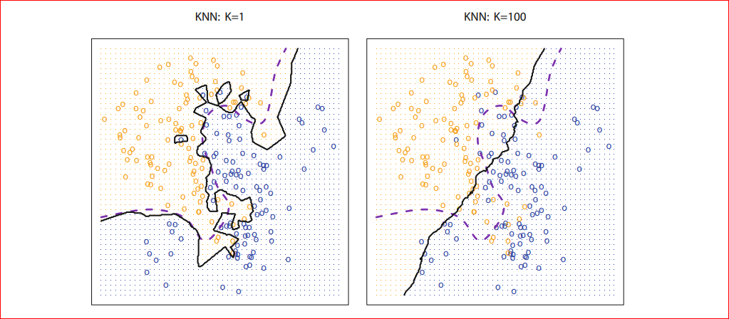 Photo credit: An Introduction to Statistical Learning with Applications in R (Available for FREE!!! )
As we can see for k=1 our decision boundary represented by black is too much fitted as k=100 we can see that our decision boundary is too much smoothed. So if k is large the decision boundary will be smoother hence a less complex model however for small k the decision boundary will less smooth and give a complex model, which will be more sensitive to the noise in the data, which may give a good prediction for training data but may fail on new data, this is also known as overfitting if we increase k too much the decision boundary will be too much smoothed (tend to become straight line) and may not perform well on both of the test and train set as can see in the figure for k=100 and this is commonly known as underfitting so we must choose k such that neither it is under fitted nor overfitted that means choose k neither too large neither too small, for k=10 we will get following
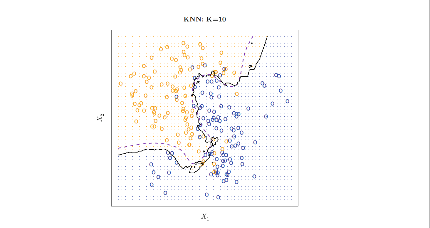 Photo credit: An Introduction to Statistical Learning with Applications in R (Available for FREE!!! )
Confusion Matrix
Accuracy is not always a good metric for measuring the performance of classification problems, suppose we have data for transactions from a bank and we have to create a model which classify whether a transaction is a fraud or not fraud, usually a lot of transactions are non-fraudulent let us say 95% are not fraudulent, this type of data is known as imbalanced data when one of the class is too frequent and for imbalanced data out accuracy metric does not perform well for imbalanced data, so there are other metrics to measure the performance of a model and they can be obtained from a very famous matrix known as Confusion Matrix
In Binary Classification there are two classes Positive and Negative, we call those classes positive class which we are interested in, suppose we want to model a transaction fraud then we are interested in the transactions which are fraud, then the class fraud is positive class and non-fraud class is negative, Various Metric can be calculated by By the Following Formulas
.png)
F1- Score can also be interpreted as Harmonic Mean of Precision and Recall , and given by
\[F1 \ Score = 2 \cdot \frac{precision \cdot recall}{precision + recall}\]Confusion Matrix can be calculated
- import confusion_matrix method from sklearn.metrics
- use confusion_matrix ,with a first argument actual test labels and second argument as prediction of the lebels
from sklearn.metrics import confusion_matrix
print(confusion_matrix(y_test,X_test_prediction))
[[13  0  0]
 [ 0 13  0]
 [ 0  1 11]]
Here we got $3\times 3 $ matrix because we have 3 classes , we are not limited to only two class positive negative, here we have three classes of labels i.e ‘versicolor’, ‘setosa’, ‘virginica’, now to get the performance metrics we have to run the following codes
from sklearn.metrics import classification_report
print(classification_report(y_test,X_test_prediction))
              precision    recall  f1-score   support

           0       1.00      1.00      1.00        13
           1       0.93      1.00      0.96        13
           2       1.00      0.92      0.96        12

    accuracy                           0.97        38
   macro avg       0.98      0.97      0.97        38
weighted avg       0.98      0.97      0.97        38
Regression
In regressions target variable is a continuous variable as price of a mobile,temperature and etc. To get started let us took diabetese dataset , which is already persent in sklearn module
from sklearn import datasets
import pandas as pd
import numpy as np
boston = datasets.load_boston()
Let us take a look at what we have imported in data variable using .keys() attribute
boston.keys()
dict_keys(['data', 'target', 'feature_names', 'DESCR', 'filename'])
Now we have data and the feature names , so we can create a dataframe from the data and feature names and can take a look at the from the head method, as we have done in Classification
X = boston.data
y = boston.target
df = pd.DataFrame(X , columns = boston.feature_names)
df.head()
| CRIM | ZN | INDUS | CHAS | NOX | RM | AGE | DIS | RAD | TAX | PTRATIO | B | LSTAT | |
|---|---|---|---|---|---|---|---|---|---|---|---|---|---|
| 0 | 0.00632 | 18.0 | 2.31 | 0.0 | 0.538 | 6.575 | 65.2 | 4.0900 | 1.0 | 296.0 | 15.3 | 396.90 | 4.98 |
| 1 | 0.02731 | 0.0 | 7.07 | 0.0 | 0.469 | 6.421 | 78.9 | 4.9671 | 2.0 | 242.0 | 17.8 | 396.90 | 9.14 |
| 2 | 0.02729 | 0.0 | 7.07 | 0.0 | 0.469 | 7.185 | 61.1 | 4.9671 | 2.0 | 242.0 | 17.8 | 392.83 | 4.03 |
| 3 | 0.03237 | 0.0 | 2.18 | 0.0 | 0.458 | 6.998 | 45.8 | 6.0622 | 3.0 | 222.0 | 18.7 | 394.63 | 2.94 |
| 4 | 0.06905 | 0.0 | 2.18 | 0.0 | 0.458 | 7.147 | 54.2 | 6.0622 | 3.0 | 222.0 | 18.7 | 396.90 | 5.33 |
Before Training the model let us split our data , we can not use stratify attribute here because our target varible is not categorical.
X_train , X_test , y_train , y_test = train_test_split(X,y,test_size = 0.25 )
Linear Regression
When we assume the target variable y is a linear function of columns of X, or we can say linear functions of features the model is known as linear regression, it can be represented as
\[\hat{y}_i = \sum_{i=0}^p a_{i}x^{i}\]Linear regression is an equation of line,and $a_i$ are known as parameters of linear regression.
Now our main aim is to set $ a_i $ such as the predicted value of y generally represented by is nearest to the actual value of y, to measure the amount of difference between the predicted and actual we use loss functions, these are a special type of functions which give 0 when the predicted value for the label is equal to the actual label, one of the most common loss function is squared error loss function given by
\[Loss(\hat{y} ;y)= \sum_{i=0}^n(y_i - \hat{y}_i)^{2}\]So our problem is to reduce loss, so to reduce we have to set optimized parameters which reduce loss, but for this type of loss the Estimation of the parameters that are $a_i$ are known as a least square estimate, for a different type of loss functions we can get different types estimate,but least square estimates are most used so we are gonna discuss this
p is the number of features , hence there will be (p+1) parameters , where we added 1 due to the fact that we have to also estimate the constant term $a_0$ and “n” is the number of observations , or we can say number of rows in the dataset
Now to fit the model , we will run the following code
from sklearn.linear_model import LinearRegression
model = LinearRegression()
model.fit(X_train,y_train)
LinearRegression(copy_X=True, fit_intercept=True, n_jobs=None, normalize=False)
Now we can predict using .predict method as follows
prediction=model.predict(X_test)
As we have seen the metric to measure the performance of a model is Accuracy in the classification section however for regression we can not use Accuracy one of the mostly used metric for regression is $R^2$ which is defined as proportion of variability in Y that can be explained using X , it can be calculated by following code
model.score(X_test,y_test)
0.736994702163782
Generally $R^2$ range vary from 0 to 1. When $R^2$ is near to 1 it represent that the model is good and when it is near to 0 the model fitted is not good
Cross Validation
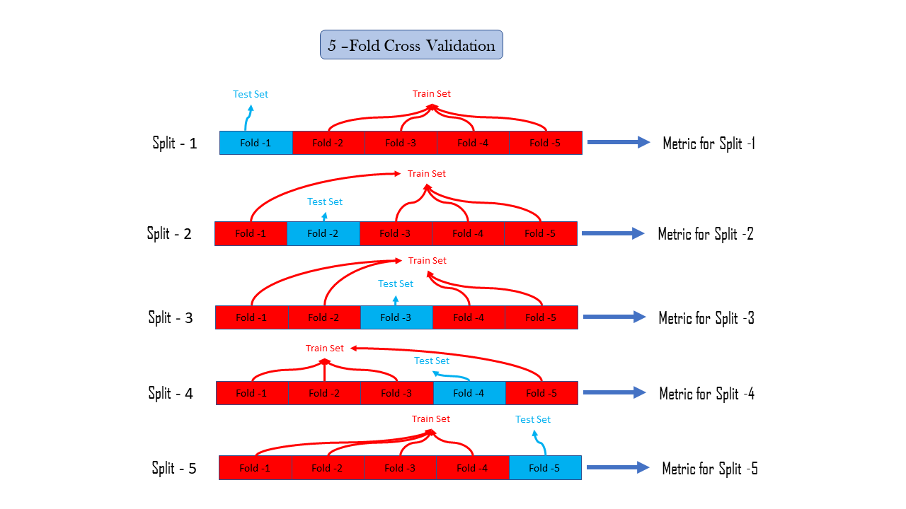
Cross-Validation is a method that reduces our dependency on how the data splits in train and test, there may be, only by chance that our performance metrics are representing our model as good, this is due to the fact we do not use all the data to calculate performance metrics. To eradicate the dependency on only one train test splits data we use Cross-Validation, or we can say k-fold Cross-validation where is k is a parameter and a positive integer suppose k=5 means there are 5-fold cross-validation, it simply divide our observations in our dataset into 5 groups commonly known as a fold, then we hold the first fold as a test set and all other folds are merged to create train set and then we calculate the performance metric we are interested in, and then do the same again by holding second fold as a test set and remaining as train set and after that calculate performance metric, this is known as a performance metric for the second split, similarly in k fold cross validation we calculate performance metric k times for k splits and further after calculating metric for every split we can calculate statistics of our interest such as the mean of these k performance metrics or mode, median or whatever statistic we want
k-Fold Cross Validation is computationally expensive , since we have to do the whole process of training, prediction and metric calculation k times , following is the way to do so
- Import
cross_val_score - call the
cross_val_scorewith arguments the model , features array , labels , number of fold suppose for 5 foldcv=5, and store it in a variable - Call the statistics function such as mean or mode on the variable such as
np.mean()for mean
from sklearn.model_selection import cross_val_score           #Importing class
cross_validation_result = cross_val_score(model,X,y,cv=5)     #Initializing
np.mean(cross_validation_result)
0.3532759243958772
Shrinkage Method
Shrinkage is also known as Regularization, In general, we estimate the parameters , but sometimes they are two large and lead to higher variance so it is advisable to shrink the parameters toward 0, it can be done in various ways two of the famous one is Ridge Regression and Lasso
Ridge Regression
For Ridge Regression we just edit our general Loss function as following
\[Loss(y \ ; \hat{y}) = \sum_{i=0}^n (y_i-\hat{y}_i)^2 + \alpha \sum_{i=1}^p a_i^2\]Where $\alpha \geq 0$ is a tuning parameter and $\alpha \sum_{i=1}^p a_i^2$ is known as shrinkage penalty, here we must note that we have not the term for in the shrinkage penalty, unlike Least Square Estimate here we get different sets of parameters for different value of tuning parameter, however for tuning parameter equal to zero will lead to Least Square Estimate and may have a greater chance of overfitting, and a very large tuning parameter will penalize the parameters too much which can lead to underfitting so we have to choose tuning parameter such as it optimizes our model
To do Ridge Regression
- Import
Ridgefrom the module sklearn.linear_model - Then initialize
Ridge()class , with passing the tuning parameter toalphaargument - Then Train and predict as usual
from sklearn.linear_model import Ridge
ridge_model = Ridge(alpha= 0.9 )
ridge_model.fit(X_train,y_train)
ridge_model.score(X_test,y_test)
0.7345197081669743
Lasso Regression
Ridge Regression has a demerit that it shrinks the parameters towards 0, but never set the parameters equal to 0, there may be some features which don’t explain any variance in the label that coefficient needs to be set equal to zero, to increase the model interpretation. For Lasso, we just add modulus of the parameters at the place of the square of parameters as in Loss of Ridge Regression
\[Loss(y \ ; \hat{y}) = \sum_{i=0}^n (y_i-\hat{y}_i)^2 + \alpha \sum_{i=1}^p |{a_i}|\]Lasso shrinks the coefficient of feature to 0 for the features which are less important
Lasso Regression have similar codes scrips as ridge Regression
from sklearn.linear_model import Lasso
lasso_model = Ridge(alpha= 10)
lasso_model.fit(X_train,y_train)
lasso_model.score(X_test,y_test)
0.7257977554026047
Logistic Regression
Logistic Regression, despite its a regression it is used in classification problem mostly, it finds out the probability that a given observation belongs to a particular class if it is greater than 0.5 or we can say 50%, then our model predict the observation label belong to that class, It estimates the probability using the following function
\[p = \sigma\left(\sum_{i=0}^p a_ix^i\right)= \frac{1}{1+ e^{-\sum_{i=0}^p a_ix^i}}\]But we will not go in theory too much, and focus on practical use. To Use Logistic Regression, it is similar to the work we have done earlier, import function, import data, split data, then test you, models, using performance metrics Let us do that, let us do this on breast cancer data, that is already available in sklearn module
from sklearn import datasets
import pandas as pd
import numpy as np
bcancer = datasets.load_breast_cancer()              #Loading Data
from sklearn.linear_model import LogisticRegression  #Importic class for logistic regression
LogReg_MODEL = LogisticRegression()                  #Initializing Logistic Regression class
X = bcancer.data
y = bcancer.target
X_train , X_test , y_train , y_test = train_test_split(X,y,test_size = 0.25 , stratify=y)  #Splitting Data
LogReg_MODEL.fit(X_train,y_train)                                                          #Training the model
AccuracyLogReg = LogReg_MODEL.score(X_test,y_test)
print(AccuracyLogReg)
0.958041958041958
ROC Curve
ROC Curve is short form for receiver operating characteristic curve.
Threshold
We generally take threshold 0.5 that means in kNN when the number of a particular class label is greater than 0.5 of the total class label we predict it belongs to that class label , suppose we fitted kNN for k=100 , and we have two class label red and blue then we will predict red for an observation if more than 50 of the neighbors are red that 50 is the threshold number , that is number of red neighbors to classify it as red , that 50 is 0.5$\times$ 100 , so here we have threshold 0.5 , similarly in logistic regression p=0.5 is threshold in general
True Positive Rate and False Positive Rate (TPR and FPR)
True Positive Rate is also known as Recall and false positive rate is given by
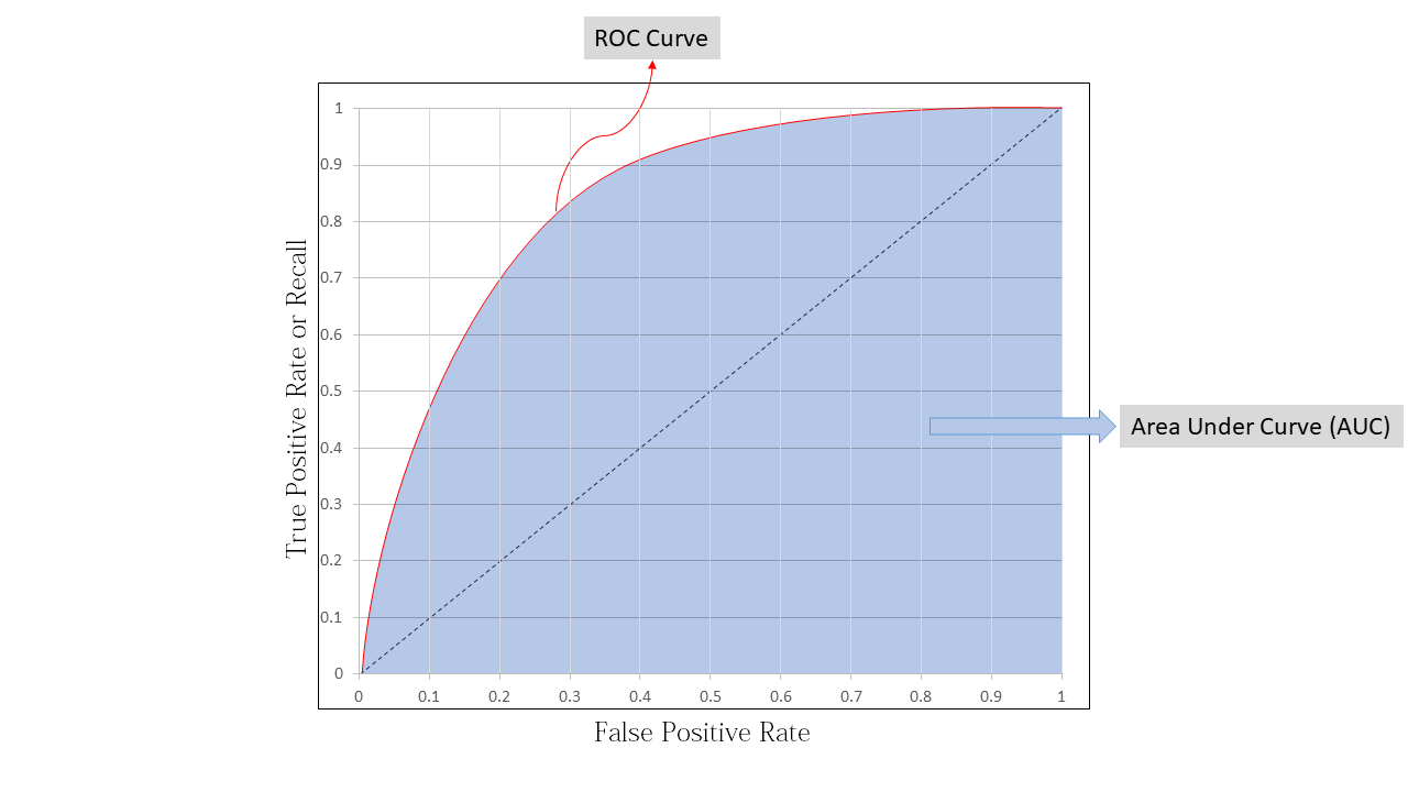
\[FPR = \frac{FP}{FP+TN}\]Model always do not perform well when the threshold is 0.5 sometimes , model performs better with threshold other than 0.5 ,to know that we use ROC curve , ROC curve is a graph between TPR and FPR and for different threshold we get different ROC curve
- When threshold is 0 , means we will predict all the observation as positive and then TPR will be equal to 1 and false positive rate will also be 1
- When threshold is 1 , both TPR and FPR will be equal to 0
To know how good is or model we use the area under curve (AUC) as a performance metric for ROC curve, lets say we have a perfect classifying model then TPR will be equal to 1 and FPR will be equal to 0 , this will be when area under the curve equal to 1 , so we can use AUC ROC as a performance metrics
Now to create ROC curve we have to do the following
- Import
roc_curvefrom sklearn.metrics - Use
roc_curve()function with following two arguments-
y_true array, shape = [n_samples]
True binary labels. If labels are not either {-1, 1} or {0, 1}, then pos_label should be explicitly given.
-
y_score array, shape = [n_samples]
Target scores, can either be probability estimates of the positive class, confidence values, or non-thresholded measure of decisions (as returned by “decision_function” on some classifiers).
-
-
Now to calculate y_score we will use probability estimates , that we can get by useing
.predict_proba()method on the test set , it will give output an array with two columns , first column is estimate and second column is probability , that is our y_score ,to get that we will subset that and take only second column by[:,1] - Further
roc_curvewill have three output , we will store those variable , FPR , TPR and thresholds - After that we will import matploblib.pyplot with alias plt and use those
.plotto plot ROC curve
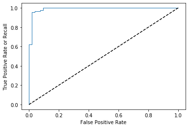
from sklearn.metrics import roc_curve
y_score = LogReg_MODEL.predict_proba(X_test)
y_score = y_score[:,1]   #Subsetting only first column
fpr, tpr, thresholds = roc_curve(y_test, y_score)


# Now to plot the ROC curve

import matplotlib.pyplot as plt
plt.plot(fpr, tpr, linewidth=1)
plt.plot([0, 1], [0, 1], 'k--')             # to plot the dashed diagonal
plt.xlabel('False Positive Rate')
plt.ylabel('True Positive Rate or Recall')
plt.show()                                  # to show the plot
Now we want performance metrics for model , and that is AUC, to calculate auc we just need to import roc_auc_score and pass the same as we passed to the roc_curve
from sklearn.metrics import roc_auc_score
print(roc_auc_score(y_test, y_score))
0.9903563941299791
Tuning the Model
Hyperparameters
Hyperparameters are the parmeters of the learning algorithm model , as for the value k in k-Nearest Neighbor model is hyperparemeter or tuning parameter in ridge and lasso regression etc. For finer model we have to tune hyperparameters to the best setting.There are not any cut and clear to go for to do hyperparameter tuning. One of the philosphy is to randomly select hyperparameters and train and test and choose one which is better. Manually fidding hyperparameters then doing the whole lot of training and testing is a tedious job to do , so Scikit Learn have a GridSearchCV to help us.
Grid Search
GridSearchCV uses cross validation so that the a hyerparameter selection is not effected by train test split.The class GridSearchCV takes the following attribute
- Model , initialized model for fitting
param_grida dictionary or a list of dictionary , this is the manual values of the hyperparameters we want to feed incvnumber of folds for cross validation
Let us tune the tuning parameter for Ridge regression model, using boston dataset
from sklearn.model_selection import GridSearchCV
knn_model = KNeighborsClassifier()
param_grid = {'n_neighbors' : [1,2,3,4,5,6,7,8,9,10,20,30,40,50,60,70,80,90,100]}
X = iris.data
y = iris.target
knn_modelGridSearch=GridSearchCV(knn_model,param_grid,cv=10)
knn_modelGridSearch.fit(X,y)
print(knn_modelGridSearch.best_score_ , ridge_modelGridSearch.best_params_)
0.9800000000000001 {'n_neighbors': 6}
Here we can see, we get best results with 6 nearest neighbors.
Now here it ends, Happy Learning
Leave a comment