Highest Posterior Density Interval

---

Highest Posterior Density Interval is interval of the parmeter in which the posterir value are high when compared to any other point outside the interval (i.e. the posterior value is high in the interval). It can be defined as a 100(1-alpha)% HPD for a parameter $\theta$ is $\mathcal{C} = { \theta : \pi(\theta \vert x) \geq k }$, where k is the largest number such that

\[\int_{\theta : \pi(\theta | x) \geq k } \pi(\theta | x) \mathrm{d} \theta = 1 - \alpha\]

Here we can think as a horizontal line in the posterior distribution, where it intersect the posterior density function such that the area under the intersection and posterior density is equal to 1-alpha.

Example

Following is a my Class assignment during my masters in the fall of 2019.

Let us consider the following dataset follows an exponential distribution with scale parameter ${\theta}$.Let us consider the prior for ${\theta}$. Obtain posterior distribution, Bayes estimator, and 0.95 HPD interval for the parameter.

3.29, 7.53, 0.48, 2.03, 0.36, 0.07, 4.49, 1.05, 9.15,3.67, 2.22, 2.16, 4.06, 11.62, 8.26, 1.96, 9.13, 1.78, 3.81, 17.02

The density of the data model will be given by

\[f(x|\theta) = \frac{1}{\theta}e^{\frac{-x}{\theta}}\]

Let us notify $\sum_{i=1}^n x_i =S_n$ now the likelihood will be given by

\[L(x|\theta) = \left(\frac{1}{\theta}\right)^ne^{\frac{-S_n}{\theta}}\]

Now Since we do not have any info about $\theta$ let us assume non-informative prior

\[\pi{(\theta)} = \frac{1}{\theta}\]

Then the posterior will be given by

\[\pi{(\theta|x)} = \frac{\frac{1}{\theta} \cdot \left(\frac{1}{\theta}\right)^ne^{\frac{-S_n}{\theta}}}{\int_0^{\infty}\frac{1}{\theta} \cdot \left(\frac{1}{\theta}\right)^ne^{\frac{-S_n}{\theta}}}\] \[\pi{(\theta|x)} = \frac{S_{n}^n}{\Gamma(n)}{ \cdot \left(\frac{1}{\theta}\right)^{n+1}e^{\frac{-S_n}{\theta}}}\]

Now this is the density of the Inverse Gamma so

\[\pi{(\theta | x)} \sim Inv-Gamma(n,S_n)\]

So the bayes estimate will be given by $\frac{S_n}{n-1}$

Code

xobs <- c(3.29, 7.53, 0.48, 2.03, 0.36, 0.07, 4.49, 1.05, 9.15,3.67, 2.22,
 2.16, 4.06, 11.62, 8.26, 1.96, 9.13, 1.78, 3.81, 17.02)
Bayes_Estimate = sum(xobs)/(length(xobs)-1) # Bayes Estimate
cat("Bayes Estimate of scale parameter is given by ",Bayes_Estimate)

## Bayes Estimate of scale parameter is given by  4.954737

Now HPDI will br given by

\[\int_{\theta : \pi(\theta|X) \geq k} \pi(\theta|X)d\theta = 1-\alpha\]

where $1- \alpha = 0.95$ , here it can be thought as a horizontal line is on the posterior density such that the point where the posterior density intersect this line the area between these points will be 0.95

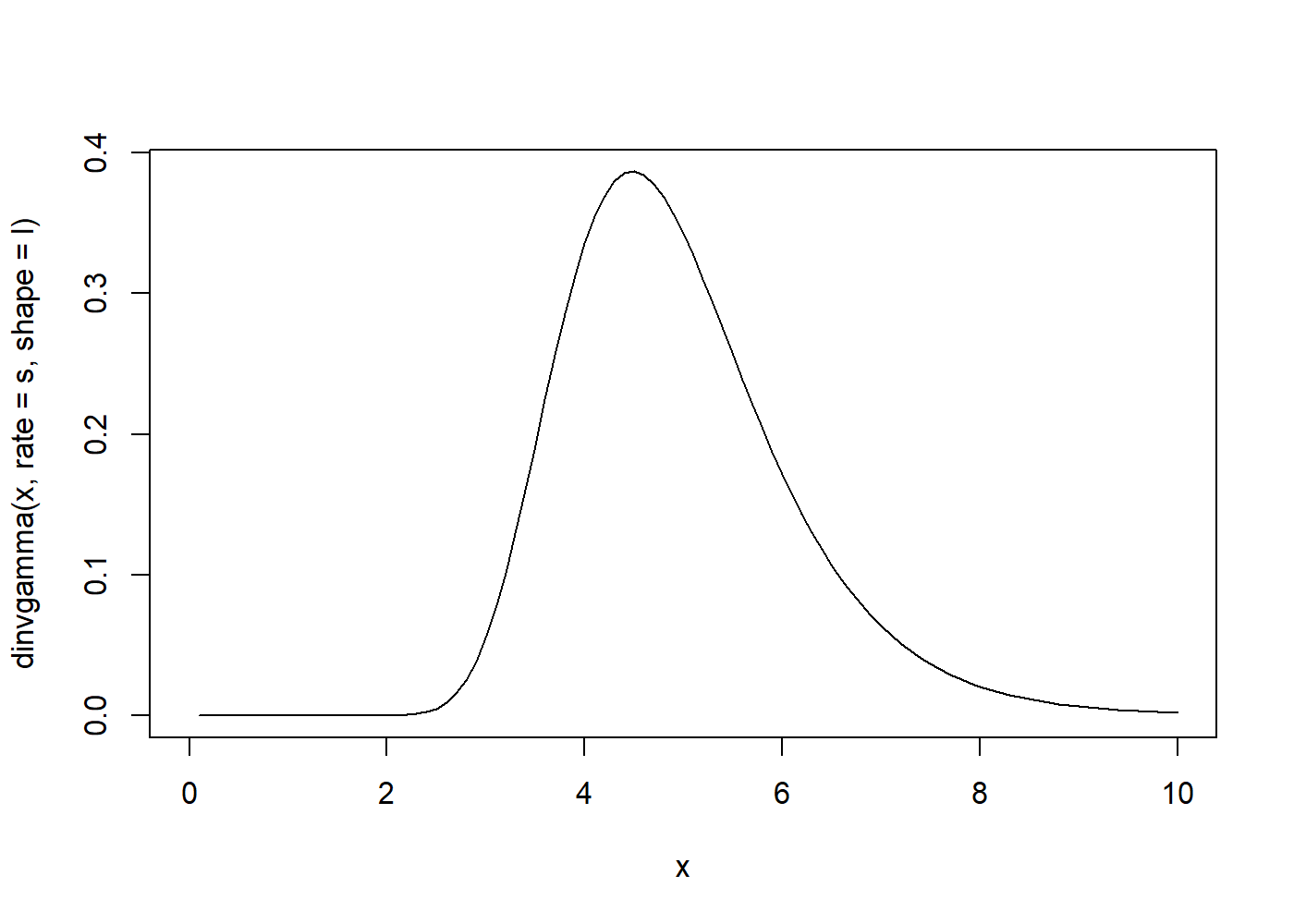
Let us take a look at posterior density function

s = sum(xobs)
l =length(xobs)
curve(dinvgamma(x , rate = s , shape = l),from=0,to=10)

Now let us find HPD , the posterior here is given by

\[\pi{(\theta|x)} = \frac{S_{n}^n}{\Gamma(n)}{ \cdot \left(\frac{1}{\theta}\right)^{n+1}e^{\frac{-S_n}{\theta}}}\]

Code for HPDI

ruler1 <- seq(2, s/(l+1),length=3500 )  #s\(l+1) is mode of posterior
ruler2 <- seq(s/(l+1), 8 ,length = 5000)
target = 0.95 
tolerance = 0.0005
done<- FALSE
for(i in ruler1)
{
  for(j in ruler2)
  {
    if(round(dinvgamma(i,rate=s,shape = l),3)==round(dinvgamma(j,rate=s,shape = l),3))
    {
      #print(paste(i,"and",j))
      L <- pinvgamma(i,rate=s,shape=l)
      H <- pinvgamma(j,rate=s,shape=l)
      if (((H-L)<(target+tolerance)) & ((H-L)>(target-tolerance)))
      { 
        done <- TRUE
        break
      }
    }
  }
 if (done){break}
}
HPD.L <- i; HPD.U <- j
print(paste(target*100, "% HPD interval:", HPD.L, "to", HPD.U))

## [1] "95 % HPD interval: 2.94588413015964 to 7.2851736061498"